Adaptive Regulation of Cassandra Repair

Repairs are one of those Cassandra jobs that everybody agrees are necessary and very few people enjoy running. If the cluster is lightly loaded and the data set is small, a repair job can look uneventful. That creates a false sense of confidence. Once the dataset grows and the cluster is carrying real production traffic, repair becomes one of the easiest ways to put the database under pressure.

Reaper had been a tool of choice for as back in the early days of Digitalis, but there were still times when repair activity pushed a cluster harder than the comfort thresholds. Repair is supposed to maintain consistency and it should not be the reason the cluster starts struggling for queries.

Cassandra repair execution model

Cassandra repair is a terminology that describes the data synchronization process that repairs any replicas that may somehow got misaligned with the other replicas. This mechanism is built into Cassandra, and is invoked through the JMX interface, usually using the nodetool command line tool. Its job is to compare replicas and reconcile differences so that replicas which should hold the same data actually do hold the same data. This process must be continuously executed in the background, especially to repair the tombstone data to be fully in sync, otherwise bad things can happen!

At the command line, the most familiar form of this is:

nodetool repair -full -pr

That command looks deceptively simple. In practice it has to be executed across the cluster. The work it triggers is substantial because each node repairs its primary-range replica data. With a full repair, the process works through the full replica data set for the tables in scope. This is not something you run on one node and then forget about.

The replica comparison is expensive because the data has to be scanned from disk and the repair process runs as fast as it is allowed to run. For each table and token range, the repair unit enters a validation stage. It generates and compares Merkle trees for the ranges in scope. It then identifies differences between replicas and streams or synchronises the missing data.

The validation stage is where operators first see the load. Merkle tree generation reads data from disk, as well as consuming CPU. If the node is already busy serving traffic or running compactions and flushes, repair starts competing with query execution for the same resources.

The effect is rarely isolated to one metric. I/O wait can rise and various threadpools can build pending tasks. Coordinator read latency may start drifting upward, while replica latency often widens before the coordinator path becomes visibly bad. If the cluster is already carrying a write-heavy or read-heavy workload, repair can add to the pressure that is already there.

This is why repair policy has to be treated as part of performance engineering rather than as a background housekeeping task.

Token-range segmentation and repair granularity

One way to avoid repair causing a long period of heavy resource usage is to work with smaller token ranges instead of treating the whole repair scope as one large unit. Cassandra has long supported token-range repair through nodetool. When using this option, instead of validating a very broad range in one go, the work is broken into smaller segments. Each segment is cheaper to validate, cheaper to reconcile and easier to schedule.

There is a simple reason this helps. Smaller segments mean smaller Merkle tree generation jobs. The read pressure is lower, the validation work is easier to spread across time, and the operator gets finer control over how fast repair progresses.

At the command line this idea is visible in token-range repair itself. A full repair of a table is conceptually very different from a repair of a bounded subrange.

nodetool repair --full my_keyspace my_table

nodetool repair -st <start_token> -et <end_token> my_keyspace my_table

In practice, repair orchestration systems use the same principle on a broader scale. They split the work into smaller ranges and move through them in a controlled way.

Segment sizing is still a balancing problem. If you create too few segments, each one is heavy and the validation stage can still hit the cluster hard. If you create too many segments, you increase orchestration overhead and spend too much time managing tiny repair units. A good repair system needs a sensible segmentation policy per table. Table size should be one of the inputs that drives that policy.

Limitations of fixed segmentation and static scheduling

Segmenting the work is helpful, but segmentation on its own does not solve the operational problem.

A repair plan that is safe at 02:00 may not be safe at 10:00. A cluster that looks quiet at the beginning of the run may pick up traffic an hour later. Compaction pressure can rise halfway through the job. One noisy table can change the shape of the workload while the repair is already in progress. Fixed segmentation and fixed parallelism do not respond to those changes.

This was the limitation I kept running into. The idea of segmented repair was right, but the cluster was still being treated as if it were static. Cassandra clusters are not static. The database is serving live traffic, compactions are consuming the CPU and IO, while repairs are streaming data. The load profile can shift during the repair window.

That is the point where the problem stops being “how do I schedule repair?” and becomes “how do I regulate repair?”

Control-theory model for repair regulation

In order to overcome the above limitations, we came up with a novel approach to regulate the repair and its impact on the database query by adopting the idea of the control theory. The simplest way to explain control theory is with a thermostat at home. The thermostat has a target temperature and measures the current temperature, and compares the current state with the target and then changes the heating output accordingly. The system does not assume the house behaves the same way all day. It responds to what the measurements are showing.

The same way of thinking can be applied to Cassandra repair. With Cassandra the target is not room temperature, but the gc_grace_seconds defined for each table. In Cassandra that window is not arbitrary.

The measured state is also different. Instead of room temperature, we observe repair progress and live cluster stress. We need to know how quickly repair is actually progressing and whether the cluster is absorbing that work comfortably.

The control outputs are the knobs that repair can really change:

• pause duration between repair segments
• repair parallelism

Figure: A basic feedback loop. The + symbol is the summing point where the input and feedback are compared. A is the forward controller or gain block that drives the system output. B is the feedback block that returns part of the output so the next control decision can be adjusted.

That is the adaptation from classical control theory into a Cassandra-specific model. In practice, AxonOps Adaptive Repair does not implement a standard transfer-function approach with Laplace-domain analysis. Cassandra repair is not a clean continuous-time plant with stable and easily modelled dynamics. It is a discrete operational process with changing workloads, shifting compaction pressure, irregular segment durations, and external disturbances from live traffic. For that reason, the repair controller was implemented as a repair-specific feedback model around variables that Cassandra repair can actually influence, rather than as a textbook controller derived from standard transfer functions.

Functional requirements for adaptive repair regulation

The repair regulator needs to satisfy a few hard requirements.

1. The target repair completion time for each table must be derived from gc_grace_seconds. The repair has to complete within that time window.
2. The number of repair segments must be chosen carefully. Too few segments make each validation unit too heavy. Too many create unnecessary orchestration overhead. AxonOps uses table disk usage metrics to calculate a reasonable segmentation balance.
3. Repair must slow down when the cluster becomes loaded.
4. Repair must speed up when the cluster has spare capacity and the deadline requires it.
5. The control loop must use signals that reflect real Cassandra stress rather than a single synthetic score.
6. Those signals have to be measured frequently enough that short-lived changes are visible while the repair is still running.

That last point is more important than it sounds. A control loop that only sees the cluster every 30 or 60 seconds is already lagging behind reality.

Load indicators and control-loop input signals

The repair regulator needs live signals from both Cassandra and Linux.

From Cassandra itself, the useful inputs include:

• pending threadpool metrics
• coordinator read and write latencies
• replica read and write latencies
• compaction-related pressure
• repair-related task backlogs where relevant

From the host, the useful inputs include:

• I/O wait
• CPU saturation
• disk throughput pressure
• network pressure when streaming becomes significant

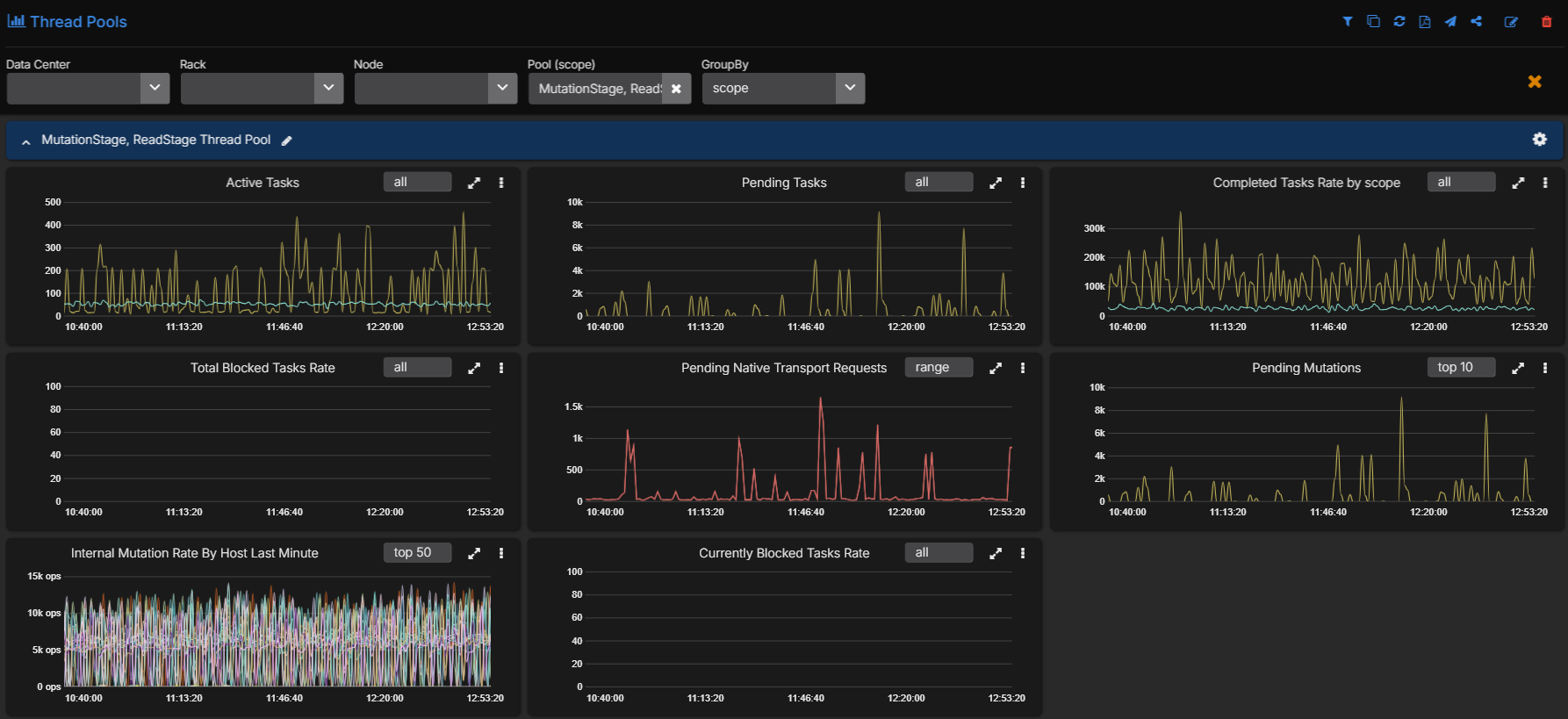
In practice, pending threadpool metrics are one of the clearest early warning signs. When MutationStage or ReadStage starts building a queue, the cluster is already telling you that the foreground request path is under pressure. That is exactly the kind of signal a repair regulator should respect. If repair continues to launch new work into that state without backing off, the cluster will absorb the extra validation and streaming load at the same time it is struggling to keep up with normal traffic.

This is exactly where high-resolution observability becomes operationally important. AxonOps collects Cassandra metrics and Linux performance metrics at 5-second resolution. That gives the repair controller a current view of the cluster rather than a delayed one. If pending tasks start climbing, coordinator latency widens, replica latency stretches or I/O wait rises, the regulator can respond while the cluster is moving into load rather than after it has already absorbed too much.

If you want the metric surface behind this in more detail, Cassandra Monitoring Best Practice Series 1: Diagnosing High Latency shows the coordinator, replica, threadpool, table, and host-level metrics that make this kind of control loop possible.

The control model

The first quantity we need is the running average repair time per completed segment:

$$\left \langle T \right \rangle = \frac{\sum_{i=0}^{n} t_i}{n}$$

Here, $n$ is the number of completed segments at the current time $t$, and $t_i$ is the time taken to repair the $i$‘th segment. This gives us the average time cost of one repair segment based on what the job has already done, not what we hoped it would do.

From there we can express the average repair velocity as segments completed per unit time:

$$\left \langle V_{segs} \right \rangle = \frac{n}{\sum_{i=0}^{n} t_i} = \frac{1}{\left \langle T \right \rangle}$$

This is the current repair velocity. It tells us how quickly the repair is actually moving.

The next quantity is the required velocity if the repair is to finish on time:

$$V' = \frac{N - n}{T - t}$$

Where $N - n$ is the number of segments still to complete, and $T - t$ is the time remaining before the deadline. This is the target velocity that the repair needs from this point onward.

If the current repair is moving too quickly for the health of the cluster, the regulator needs to add pause time between segments:

$$t_{sleep} = \frac{T - t}{N - n} - \left \langle T \right \rangle$$

That expression gives the amount of time to wait between repair segments so that repair progress stays aligned with the target end time instead of simply running flat out.

If the current repair is too slow and needs to catch up, the regulator uses parallelism instead:

$$\alpha = \frac{V'}{\left \langle V_{segs} \right \rangle}$$

Here, $\alpha$ is the repair parallelism factor. It is the ratio between the required repair velocity and the current average repair velocity.

The last piece is that the target end time cannot be treated as fixed if cluster conditions are changing materially. That is where repair strength comes in. We derive a weighted term from live metrics:

$$R_{strength} \propto \sum_{i=0}^{n}\frac{w_i}{A}\frac{M_i}{\left \langle M \right \rangle}$$

With:

$$A = \sum_{i=0}^{n} w_i$$

And:

$$\sum_{i=0}^{n}\frac{w_i}{A} = 1$$

Each live metric $M_i$ is compared with its moving average $\left \langle M \right \rangle$. If the live value is above its normal level, it contributes more pressure to the repair-strength calculation. If several signals rise together, the regulator sees that the cluster is under stress and can reduce repair intensity.

How AxonOps regulates repair in practice

The practical adaptation is straightforward even though the maths behind it is more formal.

Figure: Adaptive repair regulation across the Murmur3 token space. Completed segments sit to the left of the current state t, i=n, remaining segments sit to the right, and the controller uses the average segment repair time ⟨T⟩, sleep time t_sleep, and the final deadline T to decide how aggressively the next repair work should be launched.

AxonOps treats Cassandra repair execution across segmented token ranges as the controlled process. The target state is completion before the table-specific deadline derived from gc_grace_seconds. The measured state is repair progress, average segment completion time and live cluster load. The control error is the difference between the current repair velocity and the velocity required to complete within the remaining time budget.

From there the controller chooses between two complementary ways of adjusting repair intensity.

Pause time is recalculated continuously. If the cluster is under pressure, AxonOps will stop launching further repair work until the metric evaluations show that repair can safely proceed again. If the cluster is quiet and there is headroom, that pause time can be reduced so the repair moves faster before any change in parallelism is needed. Parallelism is then the stronger acceleration control for the cases where the repair still needs more velocity to complete within the allowed window.

Segmentation in AxonOps is part of that same regulation model rather than a separate static pre-step. The system does not hard-code one segment count for every table. It calculates segment granularity from the table volume on each node, the vnode count, the configured target segment size and a hard ceiling on the total number of segments allowed for the table.

At a high level, the embedded segmentation logic looks like this:

input:
  num_tokens_per_node
  table_volume_per_node
  target_segment_size_mb
  max_total_segments

total_table_volume_mb = sum(table_volume_per_node)
total_vnodes = node_count * num_tokens_per_node

if max_total_segments < total_vnodes:
  assign 1 segment per vnode
  return

total_segments = floor(total_table_volume_mb / target_segment_size_mb)

if total_segments > max_total_segments:
  total_segments = max_total_segments
  target_segment_size_mb = floor(total_table_volume_mb / max_total_segments)

for each node:
  node_segments = proportional_share(node_volume / total_table_volume_mb, total_segments)
  segments_per_vnode = max(1, floor(node_segments / num_tokens_per_node))
  per_segment_volume_mb = node_volume / (segments_per_vnode * num_tokens_per_node)

That gives smaller tables a simpler repair plan while larger tables get finer granularity without creating a pathological number of tiny repair units. It also means the segmentation policy is directly connected to the same repair deadline and cluster-load model that governs pause time and parallelism during execution.

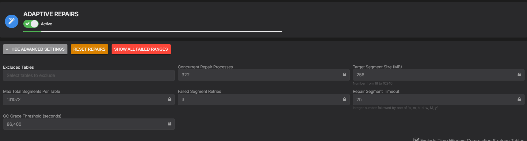
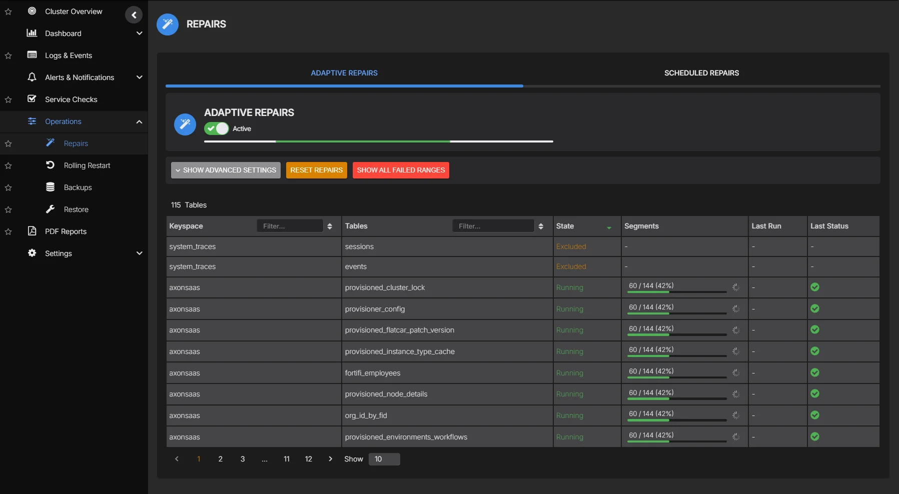
These are the policy inputs that shape how the regulator behaves in practice. Target Segment Size (MB) and Max Total Segments Per Table govern the segmentation granularity. Concurrent Repair Processes defines the upper bound the controller can work within when it needs more repair velocity. Repair Segment Timeout and Failed Segment Retries define how individual repair units are handled when they stall or fail. GC Grace Threshold (seconds) ties the whole schedule back to the anti-entropy deadline the table must satisfy.

This is not just theory or a lab model. AxonOps Adaptive Repair has been running successfully across hundreds of Cassandra clusters. Repair logic can look sensible on paper and still fail once it meets real production traffic, uneven table sizes, compaction pressure, and the day-to-day messiness of live systems. The design described here comes from running that workload at scale rather than from building a controller in isolation.

This is the part I wanted for years in repair tooling. The system should not assume that the cluster state at the start of the repair will remain valid for the full run. It should observe what is happening and adjust the launch rate of the next repair work.

5-second metrics resolution as a control-loop requirement

This kind of regulator only works if the measurements are current enough to be useful.

If pending threadpool metrics begin rising, if coordinator latency moves up, if replica latency starts widening or if host-level I/O wait climbs, the repair controller needs to see that quickly. A coarse collection interval smooths away the short-term load changes that should influence the next repair decision.

That is why the 5-second resolution in AxonOps is not just a dashboard preference. It is part of what makes adaptive repair regulation possible. The controller needs a recent view of both the database and the host. Without that, the feedback loop is too slow and the control action becomes less credible. I wrote about the sampling side of this in more detail in Time Series Metrics, Sampling Theory, and Enterprise Monitoring.

Apache Cassandra 5.0.8 and CEP-37

Apache Cassandra is now moving in this direction itself. Cassandra 5.0.8 implements the CEP-37 repair scheduler work. That is an important step for the project. Repair scheduling has been a long-standing operational gap in Cassandra. Other background maintenance tasks have always lived inside the database. Repair usually had to be driven externally by scripts, Reaper or other orchestration systems. CEP-37 changes that by introducing an in-database scheduler with node-level history, automatic execution, token-range splitting, repair metrics and guardrails around how repair runs.

That is good news for Cassandra operators. It lowers the barrier for teams that want a built-in repair mechanism rather than standing up and maintaining a separate repair stack. It also adds useful features around full and incremental repair scheduling, table-level enablement, node-level control and protective throttles.

Paul Chandler’s write-up of Cassandra Auto Repairs - Part 2 is broadly in line with that view. He calls out the separate policy controls for full and incremental repairs, node-level enablement through nodetool, built-in cluster protection and the richer repair metrics surface. He also points out some current limitations. One is the lack of time-of-day scheduling. Another is that repair interval is still effectively driven by the smallest gc_grace_seconds requirement in scope when different table classes need to coexist.

That last point is where the difference in design becomes important. CEP-37 gives Cassandra an internal scheduler and throttling controls. That is useful, but it is still fundamentally blind to the live workload. AxonOps goes further by treating repair as a feedback-regulated process using live Cassandra and Linux telemetry at 5-second resolution. The distinction is not whether repair can be split, retried or throttled. Cassandra now has those capabilities. The distinction is whether repair intensity is being adjusted continuously with cluster-level awareness of performance state. That decision is driven by live signals such as pending ReadStage and MutationStage work, replica latency drift, coordinator latency drift, I/O wait and the remaining time budget before the table-level deadline closes.

So this is not a criticism of CEP-37. It is a welcome improvement and it closes a real gap in the database. It also shows that the Cassandra project is converging on the same conclusion many operators reached years ago: repair has to be automated, observable and controlled. The AxonOps view is simply that once you accept that premise, the next logical step is adaptive regulation driven by high-resolution telemetry rather than static scheduling alone.

Closing

Repair has always been necessary in Cassandra. The hard part has been making it predictable under real production load.

Segmenting repair token ranges was an important step because it reduced the size of each repair unit and made scheduling more flexible. It did not solve the larger problem on its own because a Cassandra cluster is not static while repair is running. Query load changes. Compaction pressure changes. The repair system has to respond to that reality.

The control-theory approach gave us a practical way to frame the problem. The repair process needs a target completion window derived from gc_grace_seconds, a current view of repair progress, and a current view of cluster stress. With those inputs, repair velocity can be regulated through pause time and parallelism so the database stays stable while repair continues to make progress.

That is the basis of AxonOps adaptive repair: a repair-specific feedback model inspired by control-theory principles and built on high-resolution Cassandra and Linux metrics, so repair can complete inside the required window without treating the cluster as if it were idle all the time. It is also already repairing hundreds of Cassandra clusters successfully in production.

If you want to see this working on your own Cassandra estate, sign up for AxonOps and connect your existing cluster. It is the easiest way to see how adaptive repair behaves against live cluster conditions instead of static repair scheduling.